HugeCTR Embedding Training Cache
Introduction to the HugeCTR Embedded Training Cache
This document introduces the Embedding Training Cache (ETC) feature in HugeCTR for incremental training. The ETC allows training models with huge embedding tables that exceed the available GPU memory in size.
Normally, the maximum model size in HugeCTR is limited by the hardware resources. A model with larger embedding tables will of course require more GPU memory. However, the amount of GPU’s and, therefore, also the amount of GPU memory that can be fit into a single machine or a cluster is finite. This naturally upper-bounds the size of the models that can be executed in a specific setup. The ETC feature is designed to ease this restriction by prefetching portions of the embedding table to the GPU in the granularity of pass as they are required.
The ETC feature in HugeCTR also provides a satisfactory solution for incremental training in terms of accuracy and performance. It currently supports the following features:
The ETC is suitable and supports most single-node multi-GPU and multi-node multi-GPU configurations.
It supports all embedding types available in HugeCTR, and the Norm, Raw and Parquet dataset formats.
Both, the staged host memory parameter server (Staged-PS) and the cached host memory parameter server (Cached-PS) are supported by the ETC:
Staged-PS: Embedding table sizes can scale up to the combined host memory sizes of each node.
Cached-PS: Embedding table sizes can scale up to the SSD or Network File System (NFS) capacity.
The ETC supports training models from scratch and incremental training with existing models. The latter is implemented via the
get_incremental_model()interface, which allows retrieving updated embedding features during training. For online training these updates are forwarded to the inference parameter server.We revised our
criteo2hugectrtool to support the key set extraction for the Criteo dataset. And we also provided a Parquet key set extraction script to help you get key set from NVT processed / Synthetic Parquet datasets.
Please check the HugeCTR Continuous Training Notebook to learn how the ETC can be used to accelerate continuous training. And please check the HugeCTR Embedding Training Cache Notebook for an end-to-end demo of using ETC to train a synthetic Parquet dataset.
Feature Description
As illustrated in Fig. 1, HugeCTR datasets can be composed of multiple dataset files. We refer to the training process of a single dataset file as a pass. One such pass is composed of one or more training batches.
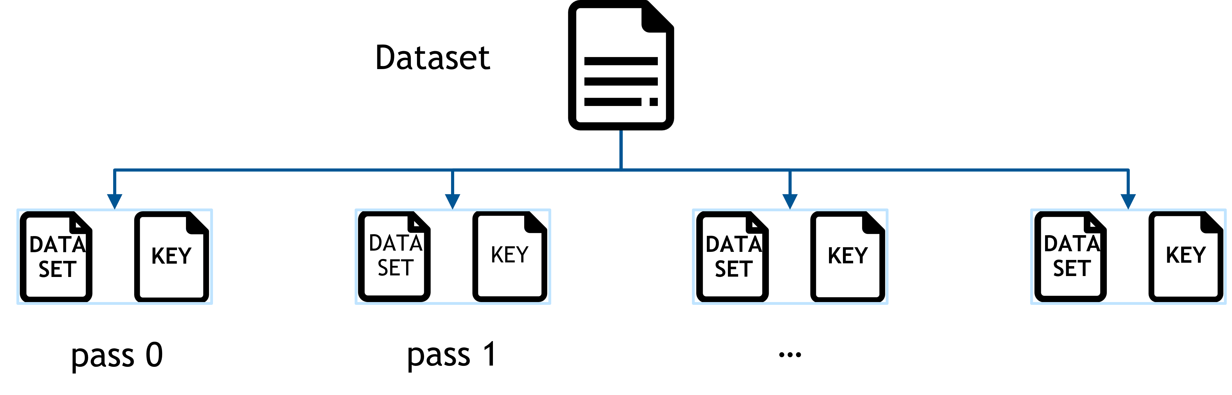
The purpose of the ETC is to prefetch required portions of the embedding table before starting a training pass. Since all features contained in the respective fetched portion of the training set are considered during training, they will also be updated during the training the pass. Hence another reason, why it can is crucial in practice to split very large datasets into multiple dataset files.
To tell the ETC which embedding features have to be prefetched for a pass, users are required to extract the unique keys from the dataset of that pass and store them into a separate keyset file (see Preprocessing for a brief file format description). Using the keyset file, the ETC calculates the total size of the embedding features to be prefetched (i.e., number of unique keys * embedding vector size), allocates memory accordingly and loads them according from the parameter server (PS).
Thereby, the ETC takes advantage of the memory compliment and inter-device communication capabilities of multi-GPU setups. All available GPU memory is used for storage, and there is no need to store duplicates of embedding features in different GPUs. Hence, the maximum size of the embedding subset to be used during a pass is just limited by the total combined memory sizes of all available GPUs.
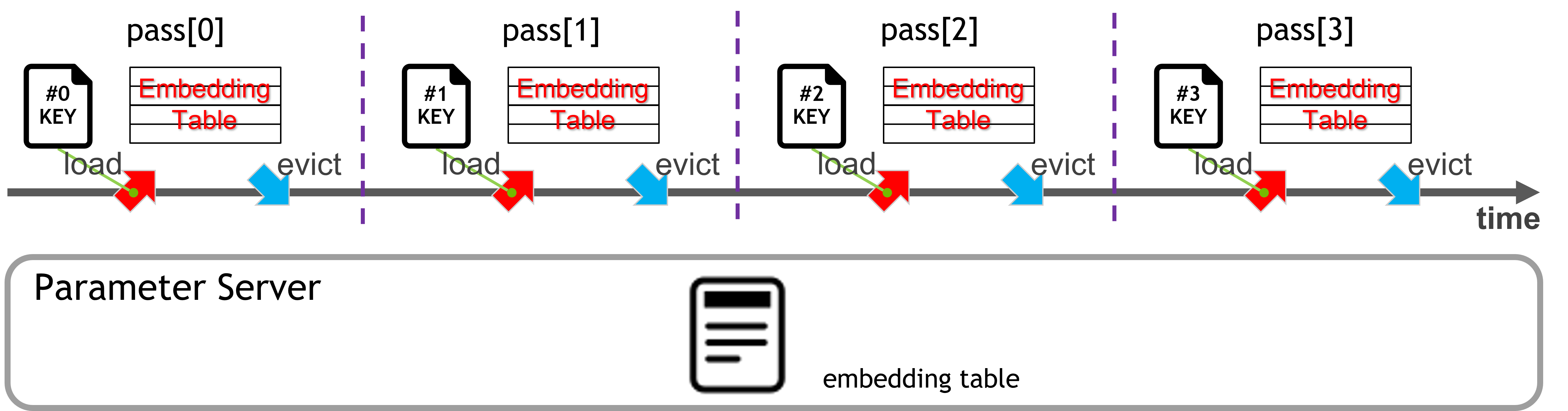
The ETC’s training process is shown in Fig. 2, in which passes are trained one by one, and each pass follows the same procedure:
Load the subset of the embedding table for the n-th pass from the PS to the GPUs.
Train the sparse and dense models.
Write the trained embedding table of the n-th pass from GPUs back to the PS.
Parameter Server in ETC
With the ETC feature, we provide two kinds of parameter servers, the staged host memory parameter server (Staged-PS) and the cached host memory parameter server (Cached-PS):
Because of its higher bandwidth and lower latency, the Staged-PS is preferable if the host memory can hold the entire embedding table.
If that is not the case, we provide the Cached-PS, which overcomes this restriction through only caching several passes’ embedding tables.
Staged Host Memory Parameter Server
The Staged-PS loads the entire embedding table into the host memory from a local SSD/HDD or a Network File System (NFS) during initialization. Throughout the lifetime of the ETC, this PS will read from and write to the embedding features staged in the host memory without accessing the SSD/HDD or NFS. After training, the save_params_to_files API allows writing the embedding table in host memory back to the SSD/HDD/NFS.
When conducting distributed training with multiple nodes, the Staged-PS utilizes the combined memories across the cluster as a cache. Thereby, it will only load subsets of the embedding table in each node, so that there are no duplicated embedding features on different nodes. Hence, for users of large models who want to use the ETC, but are stuck by the limited host memory size of a single node, increasing the number of nodes and can allow overcoming this limitation.
Since all reading and writing operations of the Staged-PS are applied within the host memory, and SSD/HDD/NFS accesses only happen during initialization and after the training has concluded. Therefore, the Staged-PS typically yields a significantly better performance than the Cached-PS in terms of the peak bandwidth.
For the configuration of a Staged-PS in a python script, please see Configuration.
Cached Host Memory Parameter Server
The Cached-PS is designed to complement the Staged-PS when an embedding table cannot fit into the host memory. The following description covers its principle, functionality, and examples of its usage. This PS is intrinsically more complex. You may skip this section, if the Staged-PS can satisfy your requirements.
Assumption
Generally speaking, the design of the Cached-PS is based on the following assumptions:
The categorical features in the dataset follow the power-law distribution and exhibit the long-tail phenomenon. Hence, there exists a small number of popular embedding features (i.e., the hot keys) will be rather frequently accessed, while the vast majority of embedding features is only occasionally required.
The composition of these hot keys may vary in actual applications. There amount may vary as well. Thus, the most recently accessed pass in the ETC may contain more or less hot keys than a previous pass.
Design of Cached-PS
We designed the Cached-PS as a custom tailored dedicated ETC-aware buffering mechanism. It is not a general-purpose software cache, and can not be generalized to other scenarios.
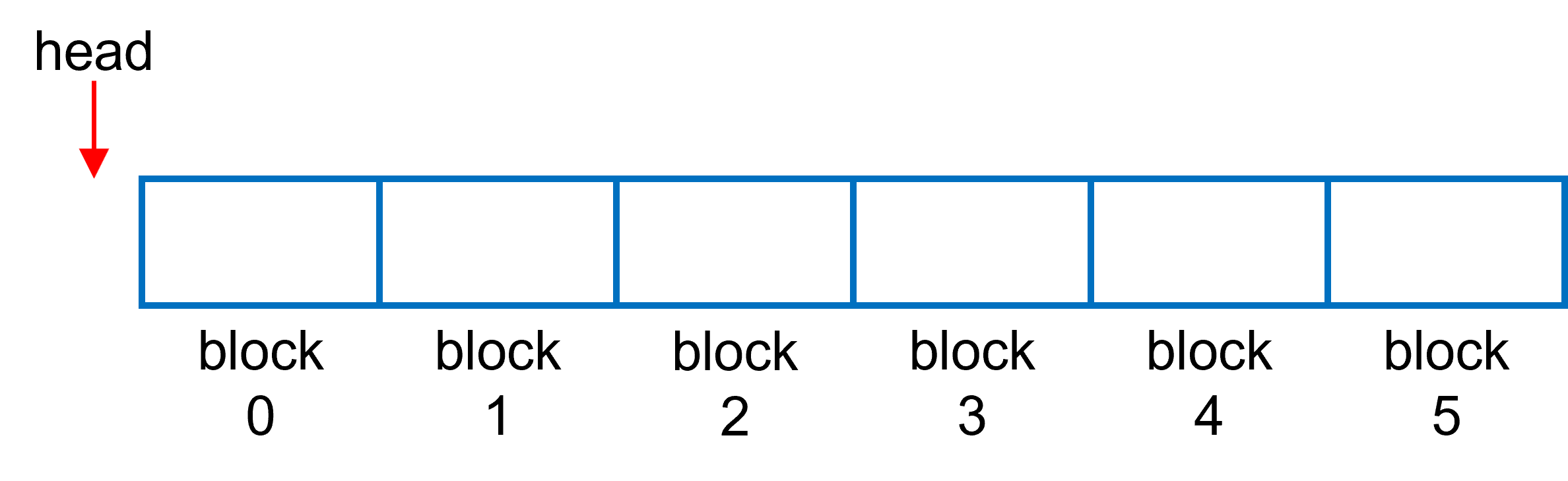
Its design aligns with the distinguishing characteristics of the ETC, which is that embeddings are transferred between host and device at the granularity of a pass. I.e., the caching granularity of the Cached-PS is the embedding table corresponding to the passes, which are marked as blocks in Fig. 3. The head marker is used to indicate the latest cached pass.
Cached-PS Configuration
The Cached-PS is configured through the following parameters:
num_blocks: The maximum number of passes to be cached (num_blocks=6in Fig. 3).target_hit_rate: A user-specified hit rate between 0 and 1. If the actual hit rate drops below this value, the ETC will attempt to migrate recently used and evict unused embeddings in the granularity of a pass.max_num_evict: The maximum number of evictions. If the number of eviction/insertion operations reaches this value, the Cached-PS will be frozen, even if thetarget_hit_rateis not yet satisfied.
The configuration API is exposed in the Python interface through the CreateHMemCache method:
hc_cnfg = hugectr.CreateHMemCache(num_blocks, target_hit_rate, max_num_evict)
The method returns a Cached-PS configuration object, hc_cnfg, corresponding to the provided values.
For example, CreateHMemCache(6, 0.6, 3) equates to a configuration, where
the Cached-PS will cache up to 6 passes,
no cache update happens if the hit rate is greater than 60%,
and the cache is frozen after at most 3 eviction/insertion operations.
Suggestions for configuration the Cached-PS for actual use-cases:
A larger number of
num_blocksis helpful to retain a high hit rate, but consumes more host memory and may cause Out of Memory issues. The upper limit value fornum_blockscan be estimated through computingavailable host memory size / embedding table size of each pass. For pointers how the latter value can be computed, please refer to Check Your Dataset.More eviction/insertion operations will happen if you set a larger value for
max_num_evict. Such operations are expensive, because they need to access the SSD/HDD/NFS. Configuring small or moderate values for this entry will improve the performance of the Cached-PS inPhase 3(see How It Works).
How It Works
We will use an example in this section to illustrate how the Cached-PS works in an actual use-case in the animation shown in Fig. 4. The configuration used for this example is CreateHMemCache(6, 0.8, 3).
The process can be divided into 3 phases:
Phase 1: Cached insertion This stage starts from the initialization if empty/unused blocks are present in the Cached-PS. When a query operation happens for a new pass, the corresponding embedding table and its optimizer states (if any) will be loaded from the SSD/HDD/NFS and inserted into an empty block. Naturally, this stage ends when as soon as all blocks of the Cached-PS are occupied (marked by
is_full=truein Fig. 2).Phase 2: Cached updating The stage starts from the end of Phase 1 (
is_full=true), and stops whennum_evict==max_num_evict. Suppose the query operation of a pass does not reach thetarget_hit_rate(80% in this example). In this case, the Cached-PS will evict the oldest block first, then load the embedding table for this new pass from both the Cached-PS (hit portion) and the SSD/HDD/NFS (missed portion), and insert it for the new pass into the available block. After each eviction/insertion operation,num_evictincreases by 1.Phase 3: Cached freezing If all blocks are occupied (
is_full==true) and the number of eviction/inseration operations reachesmax_num_evict(num_evict == max_num_evict), the cache will be frozen, and no updating will occur for later queries.
Shortcomings
To optimize throughput performance, we do not check for duplicates when storing the embedding table of a new pass into the cache block. Consequently, some portions of the embedding table are repeatedly cached, which can be considered as a drawback of the Cached-PS.
User Guide
This section gives guidance regarding the preprocessing of the dataset and how the ETC object can be configured in a Python script.
Check Your Dataset
First, you need to decide whether you need to split the dataset into sub-datasets. To do so, you need to:
Extract the unique keys of categorical features from your dataset and get the number of unique keys.
Calculate the size of the embedding table corresponding to this dataset by
Embedding Size in GB =
Factor * Num of unique keys * embedding vector size * sizeof(float) / 1024^3.Note: Beside the gradients themselves, advanced gradient-descent-based optimizers may have additional memory requirements, which are represented as the multiplicative variable
Factorin the above equation. Suggested values forFactorwhen using different optimizers available in HugeCTR are provided in Tab. 1.Compare the embedding size with the aggregated memory size of the GPUs used during training. For example, with a 8x Tesla A100 (80 GB per GPU) setup, the cumulative GPU memory size available during training is 640 GB. If the embedding size is larger than the GPU memory size, you must split the dataset into multiple sub-datasets.
Tab. 1: Suggested value for “Factor” of when using different optimizers
Optimizer |
Adam |
AdaGrad |
Momentum SGD |
Nesterov |
SGD |
|---|---|---|---|---|---|
Factor |
3 |
2 |
2 |
2 |
1 |
Note: Please mind that the equation above represents a crude estimation because other components (e.g., data reader, dense model, etc.) may share the GPU memory in HugeCTR. In practice, the available size for the embedding table is smaller than the aggregated size.
Preprocessing
Each dataset trained by the ETC is supposed to have a keyset file extracted from the categorical features. The file format of the keyset file as follows:
Keys are stored in binary format using the respective host system’s native byte order.
There are no separators between keys.
All keys use the same data type as the categorical features in the dataset (i.e., either
unsigned intorlong long).There are no requirements with respect to the sequential ordering. Hence, keys may be stored in any order.
If your dataset is in Parquet format, you can use this keyset generator we provided to get the keyset file.
Configuration
Before moving on, please have a look at the CreateETC() section in HugeCTR Python Interface, as it provides a description of the general configuration process of the ETC. Also, please refer to the HugeCTR Continuous Training Notebook for usage examples of the ETC in actual applications.
Staged-PS
To configure the Staged-PS, you need to provide two configuration entries: ps_types and sparse_models. Each entry is a list, and the number of entries in these lists must be equal to the number of embedding tables in your model.
For example, assume we want to train a WDL model, which contains two embedding tables. Then, we could configure to use the Staged-PS for both of these tables, using the following configuration:
etc = hugectr.CreateETC(
    ps_types = [hugectr.TrainPSType_t.Staged, hugectr.TrainPSType_t.Staged],
    sparse_models = [output_dir + "/wdl_0_sparse_model", output_dir + "/wdl_1_sparse_model"])
Cached-PS
To configure the Cached-PS, you need to provide the following 4 configuration entries: ps_types, sparse_models, local_paths and hcache_configs. The length of these entries are:
ps_types: The number of embedding tables in the model.sparse_models: The number of embedding tables in the model.local_paths: The number of MPI ranks.hcache_configs: 1 (broadcast to all Cached-PS), or the number of Cached-PS (Cached) inps_types.
Again, taking the WDL model as an example. A valid configuration of the ETC could be either of the following:
# Use the Staged-PS for the 1st and Cached-PS for the 2nd embedding table (1 MPI rank).
hc_cnfg = hugectr.CreateHMemCache(num_blocks=xx, target_hit_rate=xx, max_num_evict=xx)
etc = hugectr.CreateETC(
    ps_types = [hugectr.TrainPSType_t.Staged, hugectr.TrainPSType_t.Cached],
    sparse_models = [output_dir + "/wdl_0_sparse_model", output_dir + "/wdl_1_sparse_model"],
    local_paths = ["raid/md1/tmp_dir"], hmem_cache_configs = [hc_cnfg])

# Use Cached-PS for both embedding tables (1 MPI rank). The two Cached-PS have the same configuration.
hc_cnfg = hugectr.CreateHMemCache(num_blocks=xx, target_hit_rate=xx, max_num_evict=xx)
etc = hugectr.CreateETC(
    ps_types = [hugectr.TrainPSType_t.Cached, hugectr.TrainPSType_t.Cached],
    sparse_models = [output_dir + "/wdl_0_sparse_model", output_dir + "/wdl_1_sparse_model"],
    local_paths = ["raid/md1/tmp_dir"], hmem_cache_configs = [hc_cnfg])

# Use Cached-PS for both embedding tables (2 MPI ranks), where the two Cached-PS have different configurations.
hc1_cnfg = hugectr.CreateHMemCache(num_blocks=xx, target_hit_rate=xx, max_num_evict=xx)
hc2_cnfg = hugectr.CreateHMemCache(num_blocks=xx, target_hit_rate=xx, max_num_evict=xx)
etc = hugectr.CreateETC(
    ps_types = [hugectr.TrainPSType_t.Cached, hugectr.TrainPSType_t.Cached],
    sparse_models = [output_dir + "/wdl_0_sparse_model", output_dir + "/wdl_1_sparse_model"],
    local_paths = ["raid/md1/tmp_dir", "raid/md2/tmp_dir"], hmem_cache_configs = [hc1_cnfg, hc2_cnfg])
Parameter Server Performance
Next, we provide performance figures for the Staged-PS and the Cached-PS in an actual use-case. In these tests, the query is conducted by providing a list of keys to the PS, upon which the corresponding embedding table will be loaded into a buffer of the host memory. Write operations are applied in the reverse order of the query.
For reference, we also provide the performance data for the SSD-PS (read from and write to the SSD/HDD/NFS directly without caching in the host memory, deprecated from v3.3 release).
Test Condition
Hardware Setup
This test is performed on a single NVIDIA DGX-2 node. For more hardware specifications, please see the DGX-2 User Guide.
Logic of Test Code
In this test, we used the data for the first three days in the Criteo Terabyte Click Logs dataset. The raw dataset is divided into ten passes. The number of unique keys and corresponding embedding table sizes are shown in Tab. 2.
We chose an embedding vector size of 128. Hence, the total embedding table size is 53.90 GB. The cache configuration used in this test was CreateHMemCache(2, 0.4, 0).
Tab. 2: Number of unique keys and embedding table size of each pass with the Criteo dataset.
Pass ID |
Number of Unique Keys |
Embedding size (GB) |
|---|---|---|
#0 |
24199179 |
11.54 |
#1 |
26015075 |
12.40 |
#2 |
27387817 |
13.06 |
#3 |
23672542 |
11.29 |
#4 |
26053910 |
12.42 |
#5 |
27697628 |
13.21 |
#6 |
24727672 |
11.79 |
#7 |
25643779 |
12.23 |
#8 |
26374086 |
12.58 |
#9 |
26580983 |
12.67 |
In this test, all passes are looped over by two iterations. We first load the embedding table of the i-th pass from the PS and then write the embedding table of (i-1)-th pass back to the PS. There are total twenty reading and nineteen writing operations (no writing happens after the initial reading operation).
To make results comparable, we execute the sync && sysctl vm.drop_caches=3 command to clear the system cache before running the testing code.
Result and Discussion
The effective bandwidth (embedding size / reading or writing time) of reading and writing along with the hit rate are shown in Fig. 5 and Fig. 6, respectively.
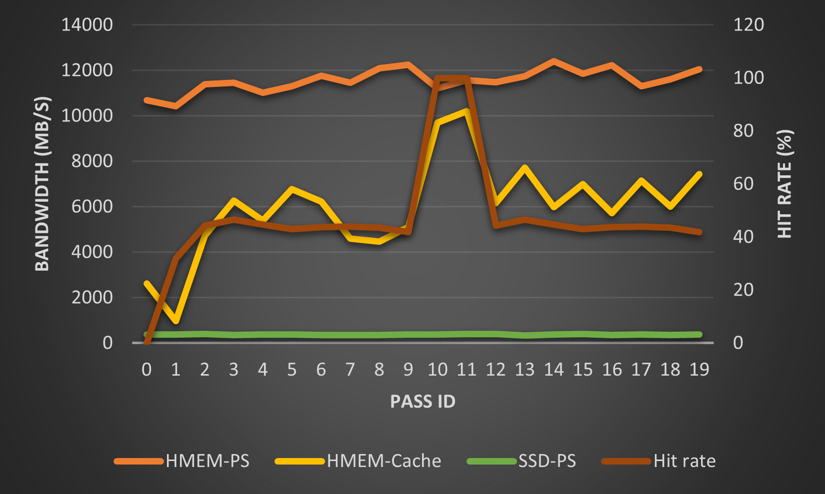
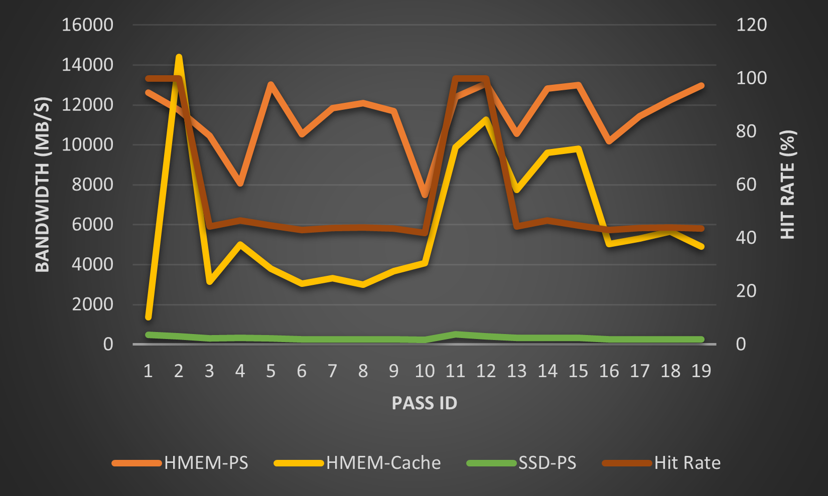
The bandwidth of the Staged-PS (=HMEM-PS) and SSD-PS (unoptimized) respectively form the upper-bound- and base-line in results. As one would expect, the bandwidth of Cached-PS (=HMEM-Cached) falls into the region between these two lines.
This embedding table of the first two passes will be cached in the HMEM-Cached. In this test we set max_num_evict=0. Thus, the cache is frozen after pass #1. For passes expect #0 and #1, both the bandwidth and hit rate fluctuate around a constant value (6000MB/s for the bandwidth, and 45% for the hit rate). The hit rate of the 10-th and 11-th reading/writing phase is 100%, because the embedding tables of the 0-th and 1-th pass are cached in the host memory. Hence, the bandwidths for these two accesses approach that of their Staged-PS counterpart.
These results show that:
In comparison to the Cached-PS, the Staged-PS provides a better and more steady performance
A properly configured Cached-PS can significantly outperform the SSD-PS (about one order of magnitude in this test).