# Copyright 2021 NVIDIA Corporation. All Rights Reserved.
#
# Licensed under the Apache License, Version 2.0 (the "License");
# you may not use this file except in compliance with the License.
# You may obtain a copy of the License at
#
#     http://www.apache.org/licenses/LICENSE-2.0
#
# Unless required by applicable law or agreed to in writing, software
# distributed under the License is distributed on an "AS IS" BASIS,
# WITHOUT WARRANTIES OR CONDITIONS OF ANY KIND, either express or implied.
# See the License for the specific language governing permissions and
# limitations under the License.
# ================================

# Each user is responsible for checking the content of datasets and the
# applicable licenses and determining if suitable for the intended use.
Taking the Next Step with Merlin Models: Define Your Own Architecture#
This notebook is created using the latest stable merlin-tensorflow container.
In Iterating over Deep Learning Models using Merlin Models, we conducted a benchmark of standard and deep learning-based ranking models provided by the high-level Merlin Models API. The library also includes the standard components of deep learning that let recsys practitioners and researchers to define custom models, train and export them for inference.
In this example, we combine pre-existing blocks and demonstrate how to create the DLRM architecture.
Learning objectives#
Understand the building blocks of Merlin Models
Define a model architecture from scratch
Introduction to Merlin-models core building blocks#
The Block is the core abstraction in Merlin Models and is the class from which all blocks inherit.
The class extends the tf.keras.layers.Layer base class and implements a number of properties that simplify the creation of custom blocks and models. These properties include the Schema object for determining the embedding dimensions, input shapes, and output shapes. Additionally, the Block has a ModelContext instance to store and retrieve public variables and share them with other blocks in the same model as additional meta-data.
Before deep-diving into the definition of the DLRM architecture, let’s start by listing the core components you need to know to define a model from scratch:
Features Blocks#
They include input blocks to process various inputs based on their types and shapes. Merlin Models supports three main blocks:
EmbeddingFeatures: Input block for embedding-lookups for categorical features.SequenceEmbeddingFeatures: Input block for embedding-lookups for sequential categorical features (3D tensors).ContinuousFeatures: Input block for continuous features.
Transformations Blocks#
They include various operators commonly used to transform tensors in various parts of the model, such as:
ToDense: It takes a dictionary of raw input tensors and transforms the sparse tensors into dense tensors.L2Norm: It takes a single or a dictionary of hidden tensors and applies an L2-normalization along a given axis.LogitsTemperatureScaler: It scales the output tensor of predicted logits to lower the model’s confidence.
Aggregations Blocks#
They include common aggregation operations to combine multiple tensors, such as:
ConcatFeatures: Concatenate dictionary of tensors along a given dimension.StackFeatures: Stack dictionary of tensors along a given dimension.CosineSimilarity: Calculate the cosine similarity between two tensors.
Connects Methods#
The base class Block implements different connects methods that control how to link a given block to other blocks:
connect: Connect the block to other blocks sequentially. The output is a tensor returned by the last block.connect_branch: Link the block to other blocks in parallel. The output is a dictionary containing the output tensor of each block.connect_with_shortcut: Connect the block to other blocks sequentially and apply a skip connection with the block’s output.connect_with_residual: Connect the block to other blocks sequentially and apply a residual sum with the block’s output.
Prediction Output Blocks#
Merlin Models provides the base ModelOutput class that consists of one head of the model. It comprises a default loss and metrics related to the given prediction task. Merlin Models provides these blocks inheriting from ModelOutput for ranking models: BinaryOutput, CategoricalOutput, andRegressionOutput.
Implement the DLRM model with MovieLens-1M data#
Now that we have introduced the core blocks of Merlin Models, let’s take a look at how we can combine them to define the DLRM architecture:
import os
import tensorflow as tf
import merlin.models.tf as mm

from merlin.datasets.entertainment import get_movielens
from merlin.schema.tags import Tags
2023-01-10 01:48:02.407367: I tensorflow/core/util/util.cc:169] oneDNN custom operations are on. You may see slightly different numerical results due to floating-point round-off errors from different computation orders. To turn them off, set the environment variable `TF_ENABLE_ONEDNN_OPTS=0`.
2023-01-10 01:48:04.740498: I tensorflow/core/platform/cpu_feature_guard.cc:193] This TensorFlow binary is optimized with oneAPI Deep Neural Network Library (oneDNN) to use the following CPU instructions in performance-critical operations:  AVX2 AVX512F AVX512_VNNI FMA
To enable them in other operations, rebuild TensorFlow with the appropriate compiler flags.
2023-01-10 01:48:06.833825: I tensorflow/core/common_runtime/gpu/gpu_device.cc:1532] Created device /job:localhost/replica:0/task:0/device:GPU:0 with 16249 MB memory:  -> device: 0, name: Quadro GV100, pci bus id: 0000:15:00.0, compute capability: 7.0
2023-01-10 01:48:06.834836: I tensorflow/core/common_runtime/gpu/gpu_device.cc:1532] Created device /job:localhost/replica:0/task:0/device:GPU:1 with 30625 MB memory:  -> device: 1, name: Quadro GV100, pci bus id: 0000:2d:00.0, compute capability: 7.0
We use the get_movielens function to download, extract, and preprocess the MovieLens 1M dataset:
DATA_FOLDER = os.getenv("DATA_FOLDER", "/workspace/data")
train, valid = get_movielens(variant="ml-1m")
We display the first five rows of the validation data and use them to check the outputs of each building block:
valid.head()
| userId | movieId | title | genres | gender | age | occupation | zipcode | TE_age_rating | TE_gender_rating | TE_occupation_rating | TE_zipcode_rating | TE_movieId_rating | TE_userId_rating | rating_binary | rating | |
|---|---|---|---|---|---|---|---|---|---|---|---|---|---|---|---|---|
| 0 | 2171 | 212 | 212 | [3, 1, 8, 2] | 1 | 1 | 5 | 1761 | -0.531961 | -0.565476 | 0.562521 | -0.715586 | -0.161680 | -0.602049 | 0 | 3.0 |
| 1 | 140 | 696 | 696 | [9, 4] | 2 | 3 | 1 | 235 | -1.102670 | 1.796455 | -0.789295 | -1.167663 | -1.261503 | -1.086495 | 0 | 3.0 |
| 2 | 345 | 944 | 943 | [3, 5] | 1 | 2 | 3 | 564 | 0.579212 | -0.608484 | 0.323336 | -1.677755 | -3.698747 | -1.434602 | 0 | 1.0 |
| 3 | 1528 | 107 | 107 | [1, 6] | 1 | 2 | 5 | 1391 | 0.597252 | -0.487549 | 0.589000 | 0.173592 | 1.103607 | 0.167345 | 0 | 2.0 |
| 4 | 749 | 577 | 577 | [1, 6] | 2 | 1 | 12 | 6 | -0.535291 | 1.796455 | 1.259219 | -0.481290 | 0.149841 | 0.614107 | 1 | 4.0 |
We convert the first five rows of the valid dataset to a batch of input tensors:
batch = mm.sample_batch(valid, batch_size=5, shuffle=False, include_targets=False)
batch["userId"]
<tf.Tensor: shape=(5, 1), dtype=int32, numpy=
array([[2171],
       [ 140],
       [ 345],
       [1528],
       [ 749]], dtype=int32)>
Define the inputs block#
For the sake of simplicity, let’s create a schema with a subset of the following continuous and categorical features:
sub_schema = train.schema.select_by_name(
    [
        "userId",
        "movieId",
        "title",
        "gender",
        "TE_zipcode_rating",
        "TE_movieId_rating",
        "rating_binary",
    ]
)
We define the continuous layer based on the schema:
continuous_block = mm.ContinuousFeatures.from_schema(sub_schema, tags=Tags.CONTINUOUS)
We display the output tensor of the continuous block by using the data from the first batch. We can see the raw tensors of the continuous features:
continuous_block(batch)
{'TE_zipcode_rating': <tf.Tensor: shape=(5, 1), dtype=float32, numpy=
 array([[-0.71558595],
        [-1.1676626 ],
        [-1.6777554 ],
        [ 0.1735921 ],
        [-0.48128992]], dtype=float32)>,
 'TE_movieId_rating': <tf.Tensor: shape=(5, 1), dtype=float32, numpy=
 array([[-0.1616803 ],
        [-1.2615032 ],
        [-3.698747  ],
        [ 1.103607  ],
        [ 0.14984077]], dtype=float32)>}
We connect the continuous block to a MLPBlock instance to project them into the same dimensionality as the embedding width of categorical features:
deep_continuous_block = continuous_block.connect(mm.MLPBlock([64]))
deep_continuous_block(batch).shape
TensorShape([5, 64])
We define the categorical embedding block based on the schema:
embedding_block = mm.EmbeddingFeatures.from_schema(sub_schema)
We display the output tensor of the categorical embedding block using the data from the first batch. We can see the embeddings tensors of categorical features with a default dimension of 64:
embeddings = embedding_block(batch)
embeddings.keys(), embeddings["userId"].shape
(dict_keys(['userId', 'movieId', 'title', 'gender']), TensorShape([5, 64]))
Let’s store the continuous and categorical representations in a single dictionary using a ParallelBlock instance:
dlrm_input_block = mm.ParallelBlock(
    {"embeddings": embedding_block, "deep_continuous": deep_continuous_block}
)
print("Output shapes of DLRM input block:")
for key, val in dlrm_input_block(batch).items():
    print("\t%s : %s" % (key, val.shape))
Output shapes of DLRM input block:
	userId : (5, 64)
	movieId : (5, 64)
	title : (5, 64)
	gender : (5, 64)
	deep_continuous : (5, 64)
By looking at the output, we can see that the ParallelBlock class applies embedding and continuous blocks, in parallel, to the same input batch. Additionally, it merges the resulting tensors into one dictionary.
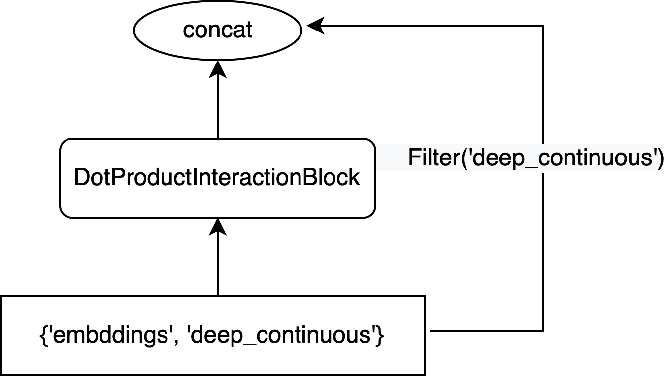
Define the interaction block#
Now that we have a vector representation of each input feature, we will create the DLRM interaction block. It consists of three operations:
Apply a dot product between all continuous and categorical features to learn pairwise interactions.
Concat the resulting pairwise interaction with the deep representation of conitnuous features (skip-connection).
Apply an
MLPBlockwith a series of dense layers to the concatenated tensor.
First, we use the connect_with_shortcut method to create first two operations of the DLRM interaction block:
from merlin.models.tf.blocks.dlrm import DotProductInteractionBlock

dlrm_interaction = dlrm_input_block.connect_with_shortcut(
    DotProductInteractionBlock(), shortcut_filter=mm.Filter("deep_continuous"), aggregation="concat"
)
The Filter operation allows us to select the deep_continuous tensor from the dlrm_input_block outputs.
The following diagram provides a visualization of the operations that we constructed in the dlrm_interaction object.
dlrm_interaction(batch)
<tf.Tensor: shape=(5, 74), dtype=float32, numpy=
array([[ 0.00000000e+00,  0.00000000e+00,  1.93288565e-01,
         0.00000000e+00,  1.85869589e-01,  9.73711610e-02,
         0.00000000e+00,  1.33227274e-01,  1.27707481e-01,
         3.35276127e-04,  0.00000000e+00,  4.16821837e-02,
         0.00000000e+00,  0.00000000e+00,  4.43421155e-02,
         1.52445361e-01,  0.00000000e+00,  0.00000000e+00,
         9.79247019e-02,  0.00000000e+00,  1.10079162e-03,
         0.00000000e+00,  2.71281973e-03,  0.00000000e+00,
         1.37151897e-01,  1.02079846e-01,  0.00000000e+00,
         7.99615458e-02,  0.00000000e+00,  9.27205235e-02,
         1.23061799e-03,  0.00000000e+00,  1.70713902e-01,
         0.00000000e+00,  8.71599466e-02,  9.89967491e-03,
         0.00000000e+00,  0.00000000e+00,  1.57242239e-01,
         1.39202520e-01,  0.00000000e+00,  2.11612321e-02,
         0.00000000e+00,  0.00000000e+00,  6.19618222e-02,
         0.00000000e+00,  0.00000000e+00,  6.24348633e-02,
         0.00000000e+00,  1.06878214e-01,  8.67929161e-02,
         0.00000000e+00,  0.00000000e+00,  1.24249667e-01,
         0.00000000e+00,  1.47114575e-01,  1.84176058e-01,
         0.00000000e+00,  0.00000000e+00,  0.00000000e+00,
         0.00000000e+00,  0.00000000e+00,  0.00000000e+00,
         0.00000000e+00,  1.58287250e-02, -2.52369717e-02,
        -7.51519576e-04, -5.56226037e-02, -9.16401204e-03,
         4.34023421e-03, -8.31933506e-03, -2.02858588e-03,
        -3.44855748e-02, -1.77974012e-02],
       [ 1.44472644e-02,  5.74837774e-02,  5.21238685e-01,
         0.00000000e+00,  3.75555277e-01,  0.00000000e+00,
         2.21605808e-01,  3.27489704e-01,  6.30696416e-02,
         0.00000000e+00,  1.29231408e-01,  1.55529499e-01,
         0.00000000e+00,  0.00000000e+00,  0.00000000e+00,
         4.20304537e-01,  0.00000000e+00,  0.00000000e+00,
         9.14298892e-02,  1.28251910e-02,  0.00000000e+00,
         0.00000000e+00,  0.00000000e+00,  0.00000000e+00,
         2.70413011e-02,  3.29245478e-01,  0.00000000e+00,
         2.87215173e-01,  0.00000000e+00,  0.00000000e+00,
         0.00000000e+00,  2.03175247e-02,  3.15539926e-01,
         0.00000000e+00,  4.37261343e-01,  4.43734266e-02,
         0.00000000e+00,  0.00000000e+00,  4.72378850e-01,
         0.00000000e+00,  0.00000000e+00,  1.28135398e-01,
         0.00000000e+00,  1.36180833e-01,  6.16933256e-02,
         0.00000000e+00,  0.00000000e+00,  0.00000000e+00,
         0.00000000e+00,  2.91504920e-01,  4.14837003e-01,
         9.94684696e-02,  0.00000000e+00,  3.01295727e-01,
         0.00000000e+00,  5.25920212e-01,  4.81699675e-01,
         0.00000000e+00,  3.81952226e-02,  0.00000000e+00,
         0.00000000e+00,  1.51182577e-01,  0.00000000e+00,
         0.00000000e+00, -4.86001372e-02, -1.03169922e-02,
         5.37233204e-02, -7.83294365e-02,  9.15671606e-03,
        -2.17590109e-03,  4.70164232e-02,  3.75321857e-03,
        -6.75947173e-04, -4.17014165e-03],
       [ 7.08196908e-02,  3.78650129e-01,  1.13808835e+00,
         0.00000000e+00,  6.76229239e-01,  0.00000000e+00,
         8.02692711e-01,  6.78692877e-01,  0.00000000e+00,
         0.00000000e+00,  7.43867755e-01,  3.88921946e-01,
         0.00000000e+00,  0.00000000e+00,  0.00000000e+00,
         9.28238153e-01,  0.00000000e+00,  3.58849168e-01,
         2.13456154e-03,  3.99174988e-01,  0.00000000e+00,
         0.00000000e+00,  0.00000000e+00,  0.00000000e+00,
         0.00000000e+00,  7.80621946e-01,  0.00000000e+00,
         7.09003448e-01,  0.00000000e+00,  0.00000000e+00,
         0.00000000e+00,  4.19765949e-01,  5.23288488e-01,
         0.00000000e+00,  1.18605947e+00,  1.17108203e-01,
         0.00000000e+00,  0.00000000e+00,  1.08671188e+00,
         0.00000000e+00,  0.00000000e+00,  3.61076236e-01,
         0.00000000e+00,  7.03222573e-01,  1.41314417e-02,
         1.45038813e-01,  0.00000000e+00,  0.00000000e+00,
         0.00000000e+00,  6.40241742e-01,  1.11257720e+00,
         5.72651088e-01,  0.00000000e+00,  6.19230390e-01,
         0.00000000e+00,  1.29610789e+00,  1.03463769e+00,
         6.19799495e-02,  4.49257553e-01,  2.95641482e-01,
         0.00000000e+00,  6.30545497e-01,  0.00000000e+00,
         0.00000000e+00, -4.93167564e-02, -3.15470368e-01,
         4.43703122e-02,  2.02106684e-02,  6.62924116e-03,
        -1.07413772e-02, -1.98644400e-02,  8.39072280e-03,
         2.27249265e-02,  1.71127990e-02],
       [ 0.00000000e+00,  0.00000000e+00,  0.00000000e+00,
         2.75904983e-01,  0.00000000e+00,  1.75966650e-01,
         0.00000000e+00,  0.00000000e+00,  1.24053761e-01,
         1.83343604e-01,  0.00000000e+00,  0.00000000e+00,
         3.19434971e-01,  7.49713704e-02,  2.17855021e-01,
         0.00000000e+00,  9.64960903e-02,  0.00000000e+00,
         4.91746925e-02,  0.00000000e+00,  1.73377842e-01,
         1.21430777e-01,  2.52151430e-01,  0.00000000e+00,
         1.76641256e-01,  0.00000000e+00,  0.00000000e+00,
         0.00000000e+00,  2.71520436e-01,  1.72208488e-01,
         9.38300714e-02,  0.00000000e+00,  0.00000000e+00,
         3.11371863e-01,  0.00000000e+00,  0.00000000e+00,
         0.00000000e+00,  2.84701586e-02,  0.00000000e+00,
         2.60322720e-01,  3.97734344e-03,  0.00000000e+00,
         0.00000000e+00,  0.00000000e+00,  2.70173680e-02,
         0.00000000e+00,  9.43048000e-02,  2.34453753e-01,
         1.85419053e-01,  0.00000000e+00,  0.00000000e+00,
         0.00000000e+00,  0.00000000e+00,  0.00000000e+00,
         1.92810968e-01,  0.00000000e+00,  0.00000000e+00,
         0.00000000e+00,  0.00000000e+00,  0.00000000e+00,
         1.20894253e-01,  0.00000000e+00,  2.14165330e-01,
         4.32761833e-02,  1.70429442e-02,  2.62627210e-02,
        -4.32948992e-02,  6.26194626e-02, -3.39646228e-02,
         1.45400483e-02,  7.81465042e-03, -8.72325525e-03,
        -4.10041586e-03, -7.54561136e-03],
       [ 0.00000000e+00,  0.00000000e+00,  7.66519830e-02,
         0.00000000e+00,  1.06283434e-01,  1.13978274e-01,
         0.00000000e+00,  6.10711798e-02,  1.23557970e-01,
         4.47871238e-02,  0.00000000e+00,  5.35226148e-03,
         0.00000000e+00,  0.00000000e+00,  8.53631198e-02,
         5.80685399e-02,  0.00000000e+00,  0.00000000e+00,
         8.35801065e-02,  0.00000000e+00,  4.29260135e-02,
         2.06196308e-02,  6.32426515e-02,  0.00000000e+00,
         1.43242419e-01,  2.64938213e-02,  0.00000000e+00,
         1.31566655e-02,  0.00000000e+00,  1.09663248e-01,
         2.36954838e-02,  0.00000000e+00,  1.05235331e-01,
         0.00000000e+00,  0.00000000e+00,  0.00000000e+00,
         0.00000000e+00,  0.00000000e+00,  4.98266704e-02,
         1.65072232e-01,  0.00000000e+00,  0.00000000e+00,
         0.00000000e+00,  0.00000000e+00,  5.18897325e-02,
         0.00000000e+00,  0.00000000e+00,  1.02630779e-01,
         0.00000000e+00,  4.15322781e-02,  0.00000000e+00,
         0.00000000e+00,  0.00000000e+00,  5.80252223e-02,
         0.00000000e+00,  2.48545967e-02,  7.69171044e-02,
         0.00000000e+00,  0.00000000e+00,  0.00000000e+00,
         0.00000000e+00,  0.00000000e+00,  0.00000000e+00,
         0.00000000e+00,  2.96171978e-02, -4.01923805e-03,
        -4.99690371e-03,  3.31057608e-02,  4.45843022e-03,
         8.83976556e-03,  2.08980199e-02, -7.50811957e-03,
        -1.51779782e-03,  1.19984746e-02]], dtype=float32)>
Then, we project the learned interaction using a series of dense layers:
deep_dlrm_interaction = dlrm_interaction.connect(mm.MLPBlock([64, 128, 512]))
deep_dlrm_interaction(batch)
<tf.Tensor: shape=(5, 512), dtype=float32, numpy=
array([[0.01001836, 0.        , 0.01265244, ..., 0.        , 0.01403767,
        0.00218583],
       [0.01719608, 0.        , 0.04947397, ..., 0.        , 0.01777297,
        0.        ],
       [0.07588126, 0.01986357, 0.18251413, ..., 0.        , 0.07191433,
        0.        ],
       [0.06161645, 0.        , 0.04086253, ..., 0.        , 0.01395844,
        0.00620432],
       [0.00864568, 0.        , 0.00794316, ..., 0.        , 0.01518907,
        0.        ]], dtype=float32)>
Define the Prediction block#
At this stage, we have created the DLRM block that accepts a dictionary of categorical and continuous tensors as input. The output of this block is the interaction representation vector of shape 512. The next step is to use this hidden representation to conduct a given prediction task. In our case, we use the label rating_binary and the objective is: to predict if a user A will give a high rating to a movie B or not.
We use the BinaryOutput class and evaluate the performances using the AUC metric.
binary_task = mm.BinaryOutput("rating_binary")
Define, train, and evaluate the final DLRM Model#
We connect the deep DLRM interaction to the binary task and the method automatically generates the Model class for us.
We note that the Model class inherits from tf.keras.Model class:
model = mm.Model(deep_dlrm_interaction, binary_task)
type(model)
merlin.models.tf.models.base.Model
We train the model using the built-in tf.keras fit method:
model.compile(optimizer="adam", metrics=[tf.keras.metrics.AUC()])
model.fit(train, batch_size=1024, epochs=1)
782/782 [==============================] - 12s 12ms/step - loss: 0.5460 - auc: 0.7847 - regularization_loss: 0.0000e+00 - loss_batch: 0.5460
<keras.callbacks.History at 0x7efc3935e130>
Let’s check out the model evaluation scores:
metrics = model.evaluate(valid, batch_size=1024, return_dict=True)
metrics
196/196 [==============================] - 2s 8ms/step - loss: 0.5355 - auc: 0.7957 - regularization_loss: 0.0000e+00 - loss_batch: 0.5356
{'loss': 0.535469651222229,
 'auc': 0.7957208752632141,
 'regularization_loss': 0.0,
 'loss_batch': 0.5560060143470764}
Note that the evaluate() progress bar shows the loss score for every batch, whereas the final loss stored in the dictionary represents the total loss across all batches.
Save the model so we can use it for serving predictions in production or for resuming training with new observations:
model.save(os.path.join(DATA_FOLDER, "custom_dlrm"))
INFO:tensorflow:Assets written to: workspace/data/custom_dlrm/assets
Conclusion#
Merlin Models provides common and state-of-the-art RecSys architectures in a high-level API as well as all the required low-level building blocks for you to create your own architecture (input blocks, MLP layers, output blocks, loss functions, etc.). In this example, we explored a subset of these pre-existing blocks to create the DLRM model, but you can view our documentation to discover more. You can also contribute to the library by submitting new RecSys architectures and custom building Blocks.
Next steps#
To learn more about how to deploy the trained DLRM model, please visit Merlin Systems library and execute the Serving-Ranking-Models-With-Merlin-Systems.ipynb notebook that deploys an ensemble of a NVTabular Workflow and a trained model from Merlin Models to Triton Inference Server.